Computer Vision for Beginners: From Pixels to Building Your Own API (OpenCV + FastAPI)

🧠 TL;DR — A digital image is just a bunch of numbers arranged in a matrix. Once that clicks, everything else in Computer Vision — grayscale, convolution, even CNNs — starts making a lot more sense. In this post we'll break the concepts down step by step, code along with OpenCV, then wrap it all into an API with FastAPI.

Ever wondered how your phone knows there's a face in a photo? Or how a CCTV system can "get suspicious" when someone walks into a restricted area? It all starts with one deceptively simple idea: a computer doesn't actually "see" an image the way we do — it just sees numbers.

Once you understand how a computer "sees" those numbers, the door into Computer Vision opens up a lot wider. Let's break it down piece by piece, with a few checkpoints along the way where you can pause and test yourself. 👇

📋 What You'll Learn

• What Computer Vision Actually Is

• Anatomy of a Digital Image

• Image Processing vs Computer Vision — What's the Difference?

• Where Computer Vision Gets Used

• Hands-On: 5 Basic Operations with OpenCV

• Bonus: Advanced Edge Detection (Sobel, Laplacian, Canny+Blur)

• From Manual Kernels to CNNs

• Wrapping It Into an API with FastAPI

• Bonus: Raw Image Endpoints & Real Deployment Proof

• Cheat Sheet & Mini Quiz

💡 If you're publishing this on Hashnode, turn on the "Table of Contents" toggle in the post settings — Hashnode auto-generates working jump-links from the headings in this article.

---

What Computer Vision Actually Is

The classic definition of AI: a system that can think and act like a human. Now, if that intelligence is pointed at language, that's NLP. If it's pointed at sight, that's Computer Vision.

💡 Computer Vision is the branch of AI that lets computers understand and interpret visual information from images or video — detecting objects, recognizing faces, even making decisions based on what it "sees."

But before a computer can "think" about an image, it needs a more basic foundation first: Image Processing. Think of it like learning a language — you can't write poetry before you know the alphabet. Image processing is that alphabet.

🧩 Quick check #1: If NLP is linguistic intelligence, what kind of intelligence is Computer Vision?

(try answering in your head before scrolling down 👇)

✅ Answer: Visual intelligence — the ability to understand information from images/video, not text.

Anatomy of a Digital Image

Here's the part people most often skip past: a digital image is a matrix of numbers.

Every image is made up of pixels — the smallest unit of an image — and each pixel holds a value representing light intensity at that point. The darker it is, the closer that value gets to 0. The brighter it is, the higher the value.

Grayscale vs RGB

	Grayscale	RGB (Color)
Number of channels	1	3 (Red, Green, Blue)
Value range per pixel	0 (black) – 255 (white)	3 values per pixel (R, G, B)
Representation	2D matrix	3D matrix (3 stacked layers)

Color is really just a combination of three numbers. For example:

• R=255, G=0, B=0 → bright red 🔴

• R=G=125, B=0 → yellowish 🟡

• R=0, G=0, B=0 → pure black ⚫

That's also why every color picker in design software shows three RGB sliders — those literally are the pixel numbers you're adjusting.

Resolution & Color Depth

A resolution of 1920 × 1080 means 1920 pixels wide and 1080 pixels tall. If it's a color image, the total number of values the computer has to store is:

1920 × 1080 × 3 channels = 6,220,800 numbers

...for just one image. That's why high-resolution images are "heavier" to process — more detail means more numbers to crunch.

Meanwhile, color depth determines how many possible color levels there are: 8-bit = 256 levels (0–255), 24-bit RGB = roughly 16 million possible color combinations.

🧮 Try it yourself: How many total numbers represent a 640×480 grayscale image?

(pause, do the math, then scroll)

✅ Answer: 640 × 480 × 1 channel = 307,200 numbers. Compare that to the color version, which needs 3× as many — 921,600 numbers! That's why converting to grayscale is a common trick for speeding up processing.

Image Dimensions: 2D vs 3D

One more characteristic that tends to get mentioned later: images also have a "dimensionality" to how they're represented.

• 2D images — grayscale, just a single layer of pixel matrix.

• 3D images — color images, where the RGB channels are stacked into one data structure (a typical shape looks like 224 × 224 × 3).

You'll run into this term a lot once you get into deep learning — especially when people talk about a model's "input shape."

Image Processing vs Computer Vision — What's the Difference?

These two terms often get used interchangeably, but they're actually different — even though they're closely related.

	Image Processing	Computer Vision
Input	Image	Image / video
Output	Image (manipulated)	Interpretation (label, coordinates, description)
Level of operation	Low-level, pixel-by-pixel	More complex and holistic
Examples	Blur, crop, edge detection	Object detection, classification, face recognition

The simple version: image processing turns an image into another image; computer vision turns an image into understanding. And usually, computer vision needs image processing as a first step before it can "understand" what's in the image.

Image processing itself covers a lot of ground — filtering, smoothing, contrast enhancement, segmentation, color transformation — and it's used widely across fields: medicine, photography, surveillance, and as the foundation for nearly every AI application that deals with visual data.

Where Computer Vision Gets Used

This isn't just theory — computer vision is already deployed across plenty of industries, often without you noticing:

🎓 Education

• Exam proctoring — detecting cheating during online exams. The system watches student behavior via webcam and flags suspicious activity like talking to someone else, looking away repeatedly, or leaving the camera frame for too long.

• Handwriting recognition — automatically grading handwritten exam answers or assignments.

🏦 Banking / Administrative

• Signature and handwriting verification on documents, for authenticity checks.

🏥 Healthcare

• Disease detection in medical imaging — scanning MRIs, CT scans, or X-rays to automatically detect things like cancer, heart abnormalities, or tumors with high accuracy.

• Microscopic image analysis — examining cells or tissue samples to spot abnormalities such as infections or pathological changes.

🏭 Manufacturing

• Automated quality inspection (visual inspection) — detecting defects, cracks, or size mismatches on the production line (a classic example: checking phone screens for defects) with speed and precision well beyond the human eye.

🔒 Security / Surveillance

• Smart surveillance — CCTV systems (including in smart cities or mining sites) detecting suspicious activity or behavior, like someone entering a restricted area.

• PPE compliance checks — automatically recognizing whether workers are wearing helmets, masks, gloves, and other required gear.

📄 Others

• OCR for document processing, and face recognition, which is now standard in plenty of everyday apps.

Almost every one of these use cases starts from the same place: processing image pixels until the computer can "read" the pattern in them.

Hands-On: 5 Basic Operations with OpenCV

Enough theory — let's write some code. We'll use OpenCV, one of the most popular Python libraries for image processing, so we don't have to implement algorithms from scratch.

⚠️ Gotcha to remember: OpenCV reads images in BGR format, not RGB! Also, coordinate (0,0) is at the top-left corner, not the center like a regular Cartesian system.

1️⃣ Image Cropping

Cropping is really just NumPy array slicing — since the image OpenCV reads is literally a 2D array.

import cv2

image = cv2.imread('input_image.jpg')

# [y_start:y_end, x_start:x_end] — rows first, then columns
cropped_image = image[50:200, 100:300]

cv2.imwrite('cropped_image.jpg', cropped_image)

2️⃣ Grayscale

import cv2

image = cv2.imread('input_image.jpg')
grayscale_image = cv2.cvtColor(image, cv2.COLOR_BGR2GRAY)
cv2.imwrite('grayscale_image.jpg', grayscale_image)

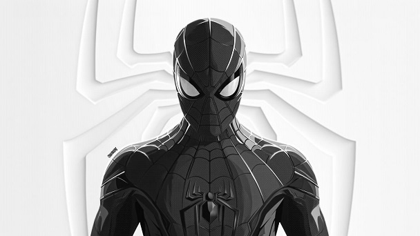
Real output from the code above — the original color image converted to black and white, keeping only light intensity.

3️⃣ Channel Split

Really handy once you get into semantic segmentation — each channel can represent a mask for a different object class.

import cv2

image = cv2.imread('input_image.jpg')
blue_channel, green_channel, red_channel = cv2.split(image)

cv2.imwrite('red_channel.jpg', red_channel)
cv2.imwrite('green_channel.jpg', green_channel)
cv2.imwrite('blue_channel.jpg', blue_channel)

4️⃣ Convolution — The Heart of Image Processing

This is the single most important concept in this whole article. Picture a kernel (a small matrix, say 5×5) sliding slowly across the image. At every position, the kernel's values get multiplied with the pixels underneath, then summed into one output value.

Different kernels = different effects:

• An averaging kernel → blur 🌫️

• Kernel [[0,-1,0],[-1,4,-1],[0,-1,0]] → edge detection ✏️

• Identity kernel → image stays unchanged

import cv2
import numpy as np

image = cv2.imread('input_image.jpg')

kernel = np.ones((5, 5), np.float32) / 25  # blur kernel
convolved_image = cv2.filter2D(image, -1, kernel)

cv2.imwrite('convolved_image.jpg', convolved_image)

🧪 Try it yourself: Swap the kernel above for the edge-detection kernel [[0,-1,0],[-1,4,-1],[0,-1,0]]. What happens?

✅ Answer: The result shows the edges of the objects in the photo, instead of a blurred whole image. That's because this kernel "highlights" the intensity differences between neighboring pixels — exactly where an object's edges are.

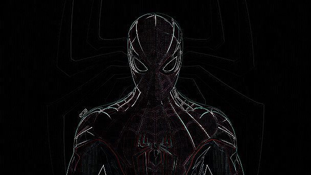
This isn't a simulation — it's the actual output of the edge-detection kernel above, applied to a Spider-Man image. Notice how the kernel "pops out" the lines of the costume.

5️⃣ Line Detection (Canny + Hough Transform)

import cv2
import numpy as np

image = cv2.imread('input_image.jpg')
gray = cv2.cvtColor(image, cv2.COLOR_BGR2GRAY)

edges = cv2.Canny(gray, 50, 150, apertureSize=3)
lines = cv2.HoughLines(edges, 1, np.pi / 180, 200)

if lines is not None:
    for rho, theta in lines[:, 0]:
        a, b = np.cos(theta), np.sin(theta)
        x0, y0 = a * rho, b * rho
        x1, y1 = int(x0 + 1000 * (-b)), int(y0 + 1000 * (a))
        x2, y2 = int(x0 - 1000 * (-b)), int(y0 - 1000 * (a))
        cv2.line(image, (x1, y1), (x2, y2), (0, 0, 255), 2)

cv2.imwrite('line_detected_image.jpg', image)

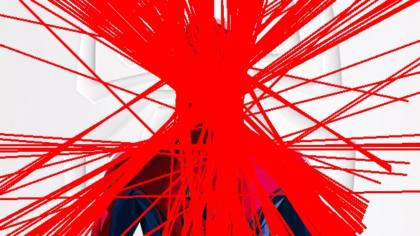
The red lines are the output of the Hough Transform — detecting straight-line patterns from the edges Canny found earlier.

How it works: Canny finds the edges first, then Hough Transform looks for straight-line patterns among those edge points — kind of like how you'd connect dots into a line yourself.

💡 Practical note: if the detected lines look too short or odd on a large-resolution image, the line length (1000 in the code above) can be made dynamic based on the image dimensions: line_length = max(img_height, img_width). The Hough Transform threshold can also be lowered (say, from 200 to 80) if too few lines are being detected.

Bonus: Advanced Edge Detection — Sobel, Laplacian & Canny + Gaussian Blur

Canny isn't the only way to detect edges. A few other variations that are commonly used:

Canny, reading straight from grayscale

import cv2

img = cv2.imread('input_image.jpg', cv2.IMREAD_GRAYSCALE)
edges = cv2.Canny(img, 100, 200)
cv2.imwrite('canny_edge_detection.jpg', edges)

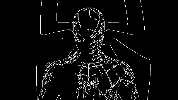
Sobel Operator — computes intensity gradients separately along the horizontal and vertical axes, then combines them into one magnitude.

sobelx = cv2.Sobel(img, cv2.CV_64F, 1, 0, ksize=3)
sobely = cv2.Sobel(img, cv2.CV_64F, 0, 1, ksize=3)

gradient_magnitude = cv2.magnitude(sobelx, sobely)
gradient_magnitude = cv2.convertScaleAbs(gradient_magnitude)
cv2.imwrite('sobel_edge_detection.jpg', gradient_magnitude)

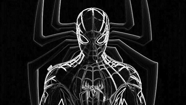
Laplacian Operator — uses the second derivative, sensitive to intensity changes in every direction at once (not just horizontal/vertical like Sobel).

laplacian = cv2.Laplacian(img, cv2.CV_64F)
laplacian_abs = cv2.convertScaleAbs(laplacian)
cv2.imwrite('laplacian_detection.jpg', laplacian_abs)

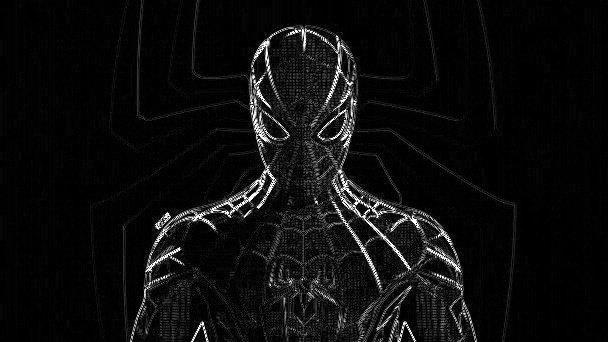
Gaussian Blur + Canny — smooth the image first before running Canny, so it doesn't pick up false edges caused by noise.

blur = cv2.GaussianBlur(img, (5, 5), 1.4)
edges = cv2.Canny(blur, threshold1=100, threshold2=200)
cv2.imwrite('canny_edge_detection_blurred.jpg', edges)

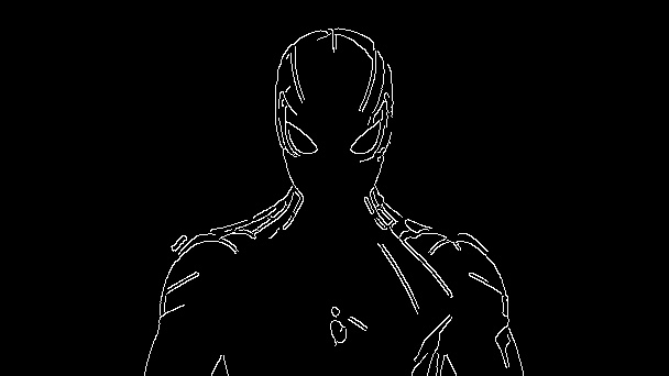
Operator	Characteristics	When to use it
Canny	Multi-stage, thin & clean edges	General edge detection, basis for Line Detection
Sobel	Separate horizontal & vertical gradients	When you need to know edge direction
Laplacian	Second derivative, sensitive in every direction	Fast, but more prone to noise
Gaussian Blur + Canny	Canny with smoothing pre-processing	Noisy images, want a cleaner result

From Manual Kernels to CNNs: The Leap That Changes Everything

Now here's the important question: how do we know what kernel values are "right" for a given task?

The answer: we don't have to define them manually. This is where Convolutional Neural Networks (CNNs) come in — instead of a kernel with fixed values, a CNN learns the best kernel values through training, adapting to whatever data it's given.

🚀 This is exactly why CNNs are so much more powerful than manual convolution: their kernels are adaptive, not hardcoded.

Architecturally, a CNN is still a regular neural network at its core — just with a series of convolutional layers added, whose job is to find the best possible values to fill those filters so that feature extraction from the image is maximized.

CNNs are a branch of deep learning built specifically for image data — a different "family" from RNNs, Transformers, or LSTMs, which are typically used for sequential data like text. If you're already familiar with those architectures from the NLP side, think of a CNN as their "cousin," purpose-built for visual data.

CNNs are a big topic on their own that we'll dig into more later — but you now know the foundation they're built on: convolution, which you just got hands-on with above.

Wrapping It Into an API with FastAPI

Finally, all five operations above can be turned into a service via an API. The idea: receive an image → process it in memory (no disk writes) → return the result as base64 — since an API endpoint can't directly return a raw image file.

Installation

pip install fastapi uvicorn pillow opencv-python

Setup & Helper Functions

from fastapi import FastAPI, UploadFile, File
from PIL import Image, ImageOps
import io, base64, cv2
import numpy as np

app = FastAPI()

def pil_image_to_base64(image: Image.Image):
    buffered = io.BytesIO()
    image.save(buffered, format="JPEG")
    return base64.b64encode(buffered.getvalue()).decode("utf-8")

def cv2_image_to_base64(image):
    _, buffer = cv2.imencode('.jpg', image)
    return base64.b64encode(buffer).decode("utf-8")

With those two helper functions, each operation just needs one endpoint:

/crop/ — crop the image to given coordinates

@app.post("/crop/")
async def crop_image(file: UploadFile = File(...), x: int = 0,
                      y: int = 0, width: int = 100, height: int = 100):
    image = Image.open(io.BytesIO(await file.read()))
    cropped_image = image.crop((x, y, x + width, y + height))
    return {"image_base64": pil_image_to_base64(cropped_image)}

/grayscale/ — convert to grayscale

@app.post("/grayscale/")
async def grayscale_image(file: UploadFile = File(...)):
    image = Image.open(io.BytesIO(await file.read()))
    grayscale_image = ImageOps.grayscale(image)
    return {"image_base64": pil_image_to_base64(grayscale_image)}

/channel_split/ — extract a single color channel

@app.post("/channel_split/")
async def channel_split(file: UploadFile = File(...), channel: str = "red"):
    image = cv2.imdecode(np.frombuffer(await file.read(), np.uint8),
                          cv2.IMREAD_COLOR)
    (blue, green, red) = cv2.split(image)
    if channel == "red":
        return {"image_base64": cv2_image_to_base64(red)}
    elif channel == "green":
        return {"image_base64": cv2_image_to_base64(green)}
    else:
        return {"image_base64": cv2_image_to_base64(blue)}

/convolution/ — apply a blur filter

@app.post("/convolution/")
async def convolution(file: UploadFile = File(...)):
    image = cv2.imdecode(np.frombuffer(await file.read(),
                          np.uint8), cv2.IMREAD_COLOR)
    kernel = np.ones((5, 5), np.float32) / 25
    convolved_image = cv2.filter2D(image, -1, kernel)
    return {"image_base64": cv2_image_to_base64(convolved_image)}

/line_detection/ — detect lines via Canny + Hough Transform

@app.post("/line_detection/")
async def line_detection(file: UploadFile = File(...)):
    image = cv2.imdecode(np.frombuffer(await file.read(),
                          np.uint8), cv2.IMREAD_COLOR)
    gray = cv2.cvtColor(image, cv2.COLOR_BGR2GRAY)
    edges = cv2.Canny(gray, 50, 150, apertureSize=3)
    lines = cv2.HoughLines(edges, 1, np.pi / 180, 200)

    if lines is not None:
        for rho, theta in lines[:, 0]:
            a, b = np.cos(theta), np.sin(theta)
            x0, y0 = a * rho, b * rho
            x1, y1 = int(x0 + 1000 * (-b)), int(y0 + 1000 * (a))
            x2, y2 = int(x0 - 1000 * (-b)), int(y0 - 1000 * (a))
            cv2.line(image, (x1, y1), (x2, y2), (0, 0, 255), 2)

    return {"image_base64": cv2_image_to_base64(image)}

Five endpoints, five image-processing operations you've learned from the ground up — and now ready to be called by anyone over HTTP. 🎉

Bonus: Raw Image Response Endpoints (Not Base64)

The five endpoints above return JSON containing base64 — a great format when the API is called from another application (web/mobile/backend), but not exactly pleasant to look at directly in a browser or Swagger UI, since it just shows up as a wall of text.

The fix is simple: build a version of each endpoint whose response is the raw image file itself (media_type="image/jpeg"), instead of JSON. Just add two helper functions to convert to raw bytes (not base64), then wrap the result in FastAPI's Response:

from fastapi.responses import Response

def pil_image_to_bytes(image: Image.Image) -> bytes:
    buffered = io.BytesIO()
    image.save(buffered, format="JPEG")
    return buffered.getvalue()

def cv2_image_to_bytes(image) -> bytes:
    _, buffer = cv2.imencode('.jpg', image)
    return buffer.tobytes()

Then build an "-image" version of each endpoint. Here's grayscale, for example:

@app.post("/grayscale-image/")
async def grayscale_image_raw(file: UploadFile = File(...)):
    image = Image.open(io.BytesIO(await file.read()))
    grayscale_image = ImageOps.grayscale(image)
    return Response(content=pil_image_to_bytes(grayscale_image), media_type="image/jpeg")

The same pattern repeats for /crop-image/, /channel_split-image/, /convolution-image/, and /line_detection-image/ — the logic is identical to the base64 versions, only the return line changes.

💡 Now your API has two "flavors" of endpoints: JSON+base64 for other programs to call, and raw image for quick testing or dropping straight into an <img src="..."> tag.

Real Proof: Deploying & Testing with ngrok

Every piece of code above has already been validated to work (tested through FastAPI's TestClient, with real requests hitting the actual endpoint functions, not just eyeballed). But beyond that — two of these endpoints (/grayscale/ and /grayscale-image/) were also tested through an actual live public deployment: the server ran on Google Colab, was exposed to the internet with ngrok, and was hit from the outside through the Swagger UI (/docs) that FastAPI generates automatically. Here's the proof:

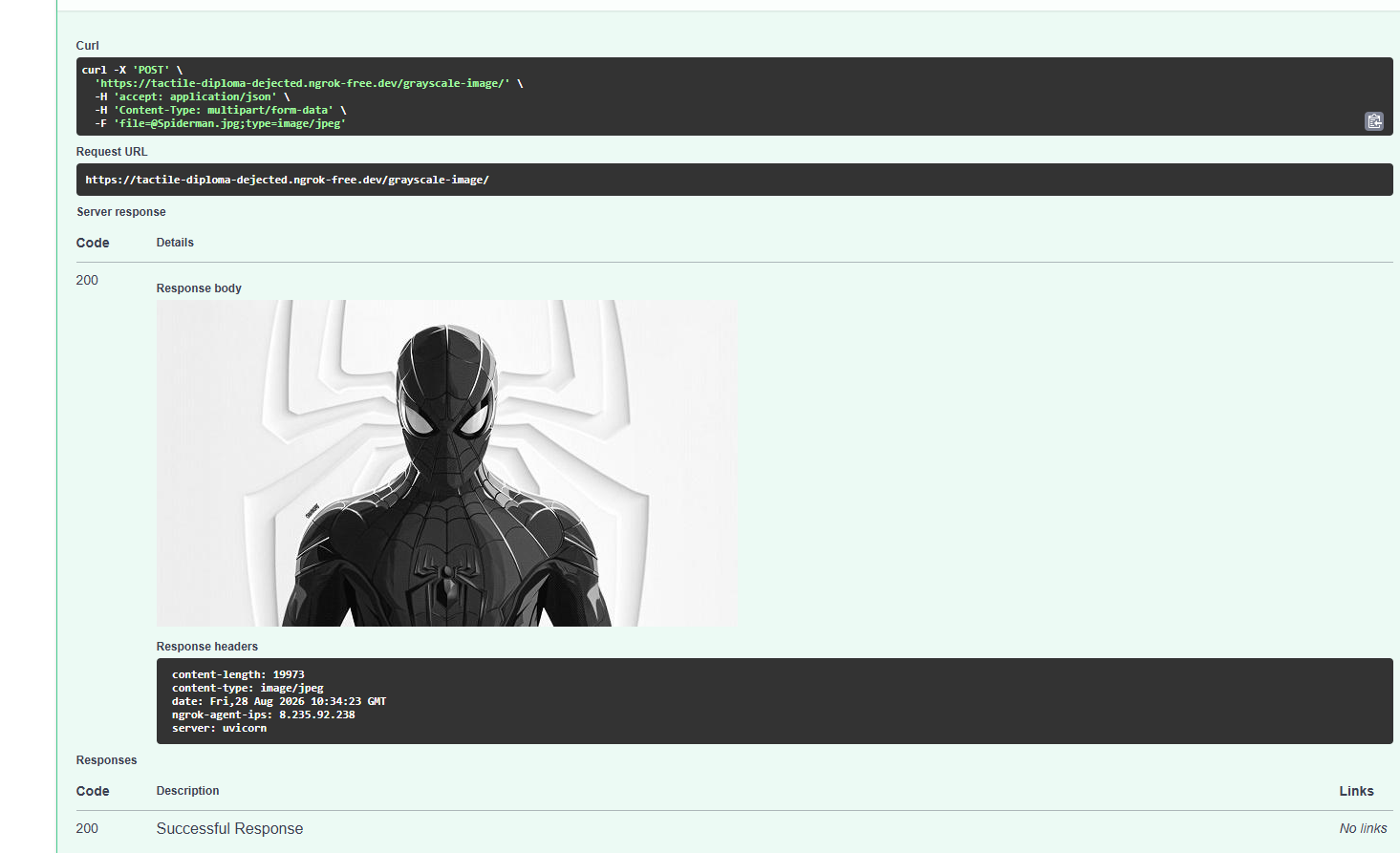
The /grayscale-image/ endpoint tested with Spiderman.jpg, with the result rendered directly as an image in the response panel. Notice the response headers: content-type: image/jpeg, server: uvicorn, and ngrok-agent-ips — proof the request genuinely went through an ngrok tunnel from the internet, not a local simulation.

If you want to try deploying your own version from Google Colab (free), here's the gist:

1. Install nest-asyncio and pyngrok.

2. Sign up for a free ngrok account and grab your authtoken from the ngrok dashboard.

3. Run uvicorn inside an asyncio.create_task() (not a plain uvicorn.run() — Colab already has its own event loop, which will conflict if you call it directly).

4. ngrok will hand you a public URL (https://xxxx.ngrok-free.dev) that tunnels to localhost:8000 on your Colab instance.

(The finer details — including a few common gotchas like port conflicts and a SystemExit that can actually crash your Colab kernel if the old server isn't shut down properly — might get their own post, since there's too much to unpack here.)

Cheat Sheet & Mini Quiz

Before you close this tab, let's consolidate everything you've learned:

Operation	What it does	Input → Output	Endpoint
Cropping	Cut out a specific area	Image → cropped image	/crop/
Grayscale	Strip out color info	Color image → black & white	/grayscale/
Channel Split	Separate R/G/B channels	1 image → 3 images, one per channel	/channel_split/
Convolution	Apply a filter via a kernel	Image → filtered image	/convolution/
Line Detection	Detect lines (Canny+Hough)	Image → image with lines marked	/line_detection/

🎯 Quick Quiz — Test Your Understanding

Try answering these three questions in your head before checking the answer under each one.

1. Why does OpenCV sometimes make image colors look "off" when displayed directly with another library?

✅ Because OpenCV reads images in BGR format, not RGB. If you display it directly with a library that assumes RGB (like matplotlib), the red and blue channels get swapped. The fix: convert it first with cv2.COLOR_BGR2RGB.

2. What's the most fundamental difference between image processing and computer vision?

✅ Image processing: image in, image out (manipulated). Computer vision: image/video in, interpretation out (labels, coordinates, descriptions).

3. Why is a CNN considered "better" than convolution with a manual (predefined) kernel?

✅ Because a CNN's kernel values are learned automatically through training and become adaptive to the data — whereas a manual kernel is fixed and requires a lot of trial-and-error to fit a specific case.

📖 Glossary of Key Terms

Bookmark this section for a quick reference whenever you forget a term:

• Pixel — the smallest unit of a digital image; its value represents light intensity at that point.

• Channel — a single matrix layer within an image (e.g., R, G, or B); the number of channels determines an image's color dimensionality.

• Resolution — the number of pixels wide × tall in an image.

• Color Depth — the number of bits used to represent each pixel's value (determines the number of possible levels/colors).

• Kernel / Filter — a small matrix slid across an image to perform a convolution operation.

• Convolution — a multiply-and-sum operation between a kernel and the overlapping image area, slid across the whole image.

• Edge Detection — a technique for detecting the edges/boundaries of objects in an image.

• Hough Transform — a method for extracting lines from edge-detection output, based on connectivity patterns between edge points.

• Semantic Segmentation — a computer vision technique for assigning a class label to every pixel in an image.

• CNN (Convolutional Neural Network) — a deep learning architecture for image data, where kernel/filter values are learned automatically through training rather than defined manually.

• Base64 — an encoding format for representing binary data (like an image) as text, commonly used when sending images through an API/JSON response.

• ngrok — a tunneling service that makes a local server (e.g., on Colab) accessible via a temporary public URL, without needing an actual cloud deployment.

---

Wrapping Up

Computer Vision looks intimidating from the outside, but once you've got the fundamentals down — pixels, matrices, and convolution — every advanced topic (CNNs, object detection, segmentation) turns out to be built on that same foundation. These same concepts will keep showing up all the way through to modern deep learning.

If you try any of the code above, share your results in the comments — I'd love to see what kernels you experimented with! 👇

Full source code (notebook, README, all verified working) is open on GitHub: github.com/arielshakaramiro/computer-vision-image-processing

---

This article is part of a learning-notes series on Computer Vision & Image Processing. Follow along for the next post in the series on Convolutional Neural Networks (CNNs).

Image credit: The Spider-Man illustration used as the example image throughout this article was sourced from Pinterest, used purely for demonstrating image-processing techniques. Spider-Man is a trademark/copyright of Marvel/Sony.

Tags: computer-vision opencv python machine-learning fastapi image-processing ai deep-learning