
Single Object Detection: Why the Bounding Box Wasn't Right

Table of Contents
📚 Computer Vision Series — Session 3. Part 3 of 3, the final part. This one runs long, and I think it's the most valuable part of the whole series.
Quick Recap
Part 2 ended with the v1 model sitting at 0.7186 test IoU. That number looks decent on paper. But once that model got tested on photos that had nothing to do with the training set, an unexpected pattern started showing up.
This part covers two more rounds of iteration (v2 and v3), the debugging in between, and one finding that changed how I read evaluation numbers from a small model like this.
Second Iteration: Augmentation and Partial Freeze
The working theory for why the bounding box sometimes came out loose: maybe the model had gotten too attached to the specific lighting conditions in the 241 training images, and stumbled whenever it hit something different.
Two changes went in together:
1. Data augmentation, train split only. ColorJitter (brightness, contrast, saturation, hue) got added so the model would learn that the same object stays the same object regardless of lighting. This augmentation was deliberately kept off the test set, so evaluation numbers stayed representative.
2. Partial backbone freeze. Instead of fine-tuning all of MobileNetV2, 14 of the first 19 blocks got frozen. The idea: general features from ImageNet pretraining are usually already reasonably robust to lighting variation, and fully fine-tuning on a small dataset (241 images) risks overwriting exactly that robustness.
class ObjectDetectionModel(nn.Module):
    def __init__(self, freeze_until=14):
        super(ObjectDetectionModel, self).__init__()
        self.backbone = mobilenet_v2(weights="DEFAULT").features
        for i, block in enumerate(self.backbone):
            if i < freeze_until:
                for param in block.parameters():
                    param.requires_grad = False
        self.classifier = nn.Sequential(
            nn.AdaptiveAvgPool2d((1, 1)),
            nn.Flatten(),
            nn.Linear(1280, 512),
            nn.ReLU(),
            nn.Linear(512, 5)
        )
    # forward() is unchanged from v1
Results:
| Metric | v1 | v2 |
|---|---|---|
| Best IoU (test) | 0.7186 | 0.7276 |
| IoU (train, final) | 0.8382 | 0.8085 |
| Train/test gap | 0.120 | 0.081 |
Test IoU inched up, but the more interesting change is the shrinking gap. v2 is less "familiar" with its own training data than v1 was, but its generalization looks healthier. On paper, this reads like a clear improvement.
🤔 Quick check: do you think v2 came out better than v1 across the board once tested on real-world photos? Click for the answer.
If you guessed "not necessarily," you'd be right. The next section shows why.
Testing the Model on Real-World Photos
The IoU numbers above come from a test set drawn from the same distribution as the training data. To get a more honest picture, the v1 model got tested on photos pulled from entirely outside the dataset, covering a much wider range of conditions.
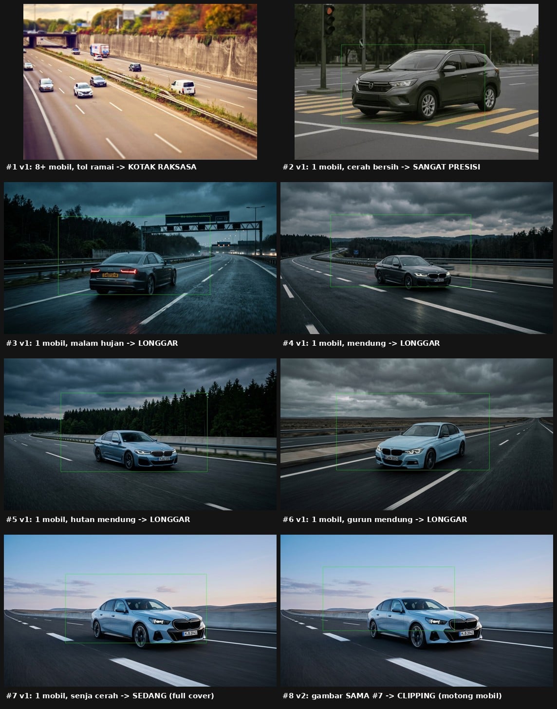
A few highlights:
A highway photo with 8+ cars at once: the model produced one oversized box spanning several cars instead of picking one. This actually makes sense. The architecture is built around a single object per image, so a busy scene throws it off.
A single car, clean background, bright daylight: the result was tight and precise, nicely wrapped around the car body.
Several single-car photos under dark or dramatically overcast skies: the results were consistently loose, boxes noticeably larger than the car and bleeding into the background.
Four out of four dark/dramatic-sky photos showed the same pattern: a loose box. The one bright, neutral-sky photo produced the tightest result of the bunch. That's consistent enough to be suspicious, though the sample size is still too small to call it a settled conclusion.
Plot Twist: A Box That Clips the Object
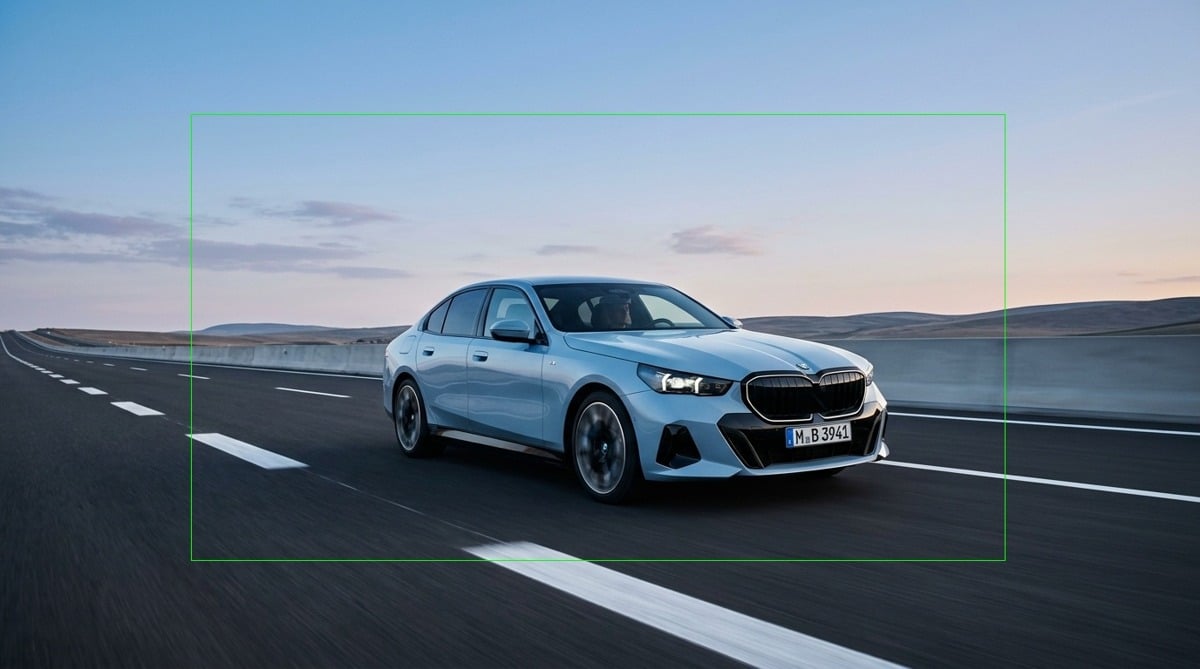
To compare v1 and v2 head-to-head, the same photo got run through both models. It happened to have a fairly bright sunset sky.
v1's result: the box fully contained the car, with a slightly loose margin above the roofline.
v2's result, on the exact same photo: the box clipped the front of the car. The bumper and part of the grille sat outside the box entirely.
That's the opposite of what you'd hope for. v2 won on the aggregate numbers (higher test IoU, smaller gap), but lost on this specific case. It's not that v2 got "worse" in some absolute sense, it traded one kind of error for a different one. A loose box is still relatively safe, the object stays fully covered. A box that clips the object is a more serious failure for anything downstream that depends on the full bounding region.
🧠 How can this happen even though the aggregate metric improved? Click for the explanation.
The test-set IoU is an average across dozens of images. An improving average doesn't guarantee better performance on every individual image, especially one (a real-world photo, not part of the original dataset) that sits far outside the training distribution. It's a useful reminder that aggregate metrics and per-case qualitative behavior are two different things, and both deserve a look.
Third Iteration: Split Head and IoU Loss
Two more changes went in, this time targeting something more fundamental: the head architecture itself.
The problem: AdaptiveAvgPool2d((1, 1)) collapses the entire feature map into a single vector before predicting the bounding box. For classification (object present or not), that's fine. For precise location regression, it's a bit like asking someone to guess where a car is in a photo after the photo's been blurred beyond recognition. The "where" information is gone before it ever reaches the part of the network responsible for predicting coordinates.
Change 1: Split head. The is_object branch keeps the 1x1 pooling, which is fine for classification. The bbox branch gets its own path that preserves a 4x4 spatial grid before the fully connected layer.
self.objectness_head = nn.Sequential(
    nn.AdaptiveAvgPool2d((1, 1)), nn.Flatten(),
    nn.Linear(1280, 256), nn.ReLU(), nn.Linear(256, 1),
)
self.bbox_head = nn.Sequential(
    nn.Conv2d(1280, 256, kernel_size=1), nn.ReLU(),
    nn.AdaptiveAvgPool2d((4, 4)), nn.Flatten(),
    nn.Linear(256 * 4 * 4, 512), nn.ReLU(), nn.Dropout(0.3), nn.Linear(512, 4),
)
Change 2: IoU loss. Added alongside MSE, not replacing it, computed with pure tensor operations so it's differentiable, and only applied to samples that actually contain an object.
@staticmethod
def _iou_loss(pred_bbox, true_bbox, eps=1e-7):
    def to_corners(box):
        x, y, w, h = box[:, 0], box[:, 1], box[:, 2], box[:, 3]
        return x - w/2, y - h/2, x + w/2, y + h/2
    px1, py1, px2, py2 = to_corners(pred_bbox)
    tx1, ty1, tx2, ty2 = to_corners(true_bbox)
    inter_w = (torch.min(px2, tx2) - torch.max(px1, tx1)).clamp(min=0)
    inter_h = (torch.min(py2, ty2) - torch.max(py1, ty1)).clamp(min=0)
    inter_area = inter_w * inter_h
    pred_area = (px2-px1).clamp(min=0) * (py2-py1).clamp(min=0)
    true_area = (tx2-tx1).clamp(min=0) * (ty2-ty1).clamp(min=0)
    union = pred_area + true_area - inter_area + eps
    return (1 - inter_area/union).mean()
This time the results were much more significant:
| Metric | v1 | v2 | v3 |
|---|---|---|---|
| Best IoU (test) | 0.7186 | 0.7276 | 0.8100 |
| IoU (train, final) | 0.8382 | 0.8085 | 0.8339 |
| Train/test gap | 0.120 | 0.081 | 0.024 |
v3 wins on both measures at once: highest test IoU, and the smallest overfitting gap of the three. On paper, it's the clear frontrunner.
Second Plot Twist: Near-Identical Boxes
The same photo that tripped up v2 got run through v3. The result: the car was fully covered again, the clipping problem was gone. But the box was now the loosest of all three versions, nearly twice the area of v1's box on that same photo.
So the pattern across versions: v1 moderately loose, v2 tight but clipping, v3 safe but the loosest yet. Three iterations, three different failure modes, not one clearly-best solution.
Then came a finding that reframed the whole picture. Two different photos got tested with v3, both under bright skies but different cars, different positions in frame:
Photo A (first car): x=686.3, y=387.2, w=932.7, h=512.0
Photo B (different car): x=685.2, y=388.0, w=938.5, h=503.3
The difference was under 1% on every coordinate. For two different cars, in different positions, in different frames.
For comparison, a third photo, dark and overcast with a completely different car and background, was also tested with v3:
Photo C (dark/overcast, different scene): x=678.5, y=385.6, w=878.5, h=485.9
Laid next to Photo A and B, this one lands in the same neighborhood too, close in both position and size, not identical, but nowhere near the dramatic swing you'd expect if lighting were driving big changes in the output. That's a stronger version of the "near-constant box" pattern than it first looked: three different cars, two very different lighting conditions, and the model's output barely moved.
(Worth noting separately: comparing v3 against v1 on that same dark photo, v1's box was noticeably smaller. So v1 and v3 clearly behave differently from each other. It's specifically v3's output across different photos that stayed this consistent.)
What This Model Might Actually Be Learning
The most plausible explanation: this model may not be genuinely tracking each object's edges on a per-image basis. It's more likely outputting something close to a default box shape and position, largely independent of what's actually in the frame. Three different cars, two very different lighting conditions, and the size and position barely moved.
This isn't a settled conclusion. Only three out-of-distribution photos were compared this closely, not a systematic study with manually annotated ground truth. But the hypothesis is consistent with everything else observed across all three versions: a total failure on a busy multi-car scene (no mechanism to pick one object among several), loose boxes that still happen to cover the object most of the time, and why fixing one failure mode through an architecture change immediately introduced a different one instead of converging toward a clean fix. A model outputting something close to a fixed guess would behave exactly like that.
If this hypothesis holds, it means the test IoU of 0.81, which looks great on paper, may actually be measuring how well that default guess happens to match the typical object size and position in the training distribution, rather than how precisely the model tracks the real edges of an object in a given photo. Those two things can produce the same number while meaning very different things.
Cheat Sheet and Takeaways
[x] v1 (baseline): full fine-tune, combined head, MSE only. Test IoU 0.7186
[x] v2: + color augmentation + partial freeze. Test IoU 0.7276, smaller gap, but a new qualitative failure (clipping) showed up
[x] v3: + split head + IoU loss. Test IoU 0.8100, smallest gap, but the loosest result on a specific qualitative test
[x] An improving aggregate metric doesn't guarantee better behavior on every individual case
[x] Working hypothesis: the model may be outputting something close to a near-constant guess, rather than precise per-object localization
[x] All code and result images are on the GitHub repo, including v2 and v3 for reference
Closing Thoughts
241 images is a small dataset, and these three iterations show its real limits. That doesn't mean the results are a failure, but it's worth reading evaluation numbers with healthy skepticism, especially for a model that hasn't been tested outside the distribution it was trained on.
If anyone wants to pick this up further, whether that's adding more data, trying a more standard grid or anchor-based architecture, or testing the "mode-based localization" hypothesis more rigorously, all the code and results are open on GitHub.
📁 Dataset: Google Drive 💻 Repo: GitHub
Closing part of the Computer Vision Super Class series, Session 3: Single Object Detection. Thanks for following along to the end.