Teaching a Computer 102 Flower Species: From Training to a Live API

The previous post covered the theory: what image classification is, how a CNN works through its backbone and head, and how to prepare a dataset. All of that stayed at the conceptual level.

This one is the hands-on half. A model gets trained to tell 102 flower species apart, from daffodils to sunflowers, using the real Oxford Flowers 102 dataset, then wrapped into an API another application can call. Every number in this post comes from an actual GPU run, not an estimate. Full code lives in the GitHub repo.

💡 Haven't read the previous post? This one assumes backbone/head and transfer learning concepts are already familiar. "Quick Recap" boxes throughout should help if not.

---

Table of Contents

1. Case Study: Oxford Flowers 102

2. Environment Setup

3. Preparing the Dataset

4. Plot Twist: A Closer Look at the Original Script

5. Building the Model with Transfer Learning

6. The Full Training Loop

7. Real Results: Accuracy, Precision, Recall

8. From Model to API with FastAPI

9. Cheat Sheet

10. Test Your Understanding

---

Case Study: Oxford Flowers 102

The dataset: Oxford Flowers 102, a collection of flower photos across 102 categories. It's a classic image classification benchmark precisely because it has so many classes, several of them visually similar to each other, the same kind of mix-up as ginger, galangal, and turmeric from the previous post, just scaled up to 102 categories.

The backbone: EfficientNet-B1, same as before. No architecture designed from scratch here, just a pretrained backbone with a swapped-out classifier.

Actual samples from the validation set, labeled using the verified cat_to_name.json mapping.

Environment Setup

pip install torch torchvision scikit-learn scipy pandas matplotlib

scikit-learn is new here, needed specifically for evaluation metrics: accuracy, precision, recall.

Preparing the Dataset

Flowers 102 doesn't come as a neat folder-per-class structure like the previous post's examples. Labels live in a separate .mat file (imagelabels.mat). This is a good opportunity to build a custom Dataset, the same pattern as the CSV approach covered earlier, just with a different label source.

import os
import torch
from torch.utils.data import Dataset, DataLoader
from torchvision import transforms
from PIL import Image
import scipy.io

class FlowersDataset(Dataset):
    def __init__(self, img_dir, all_files, labels, indices, transform=None):
        self.img_dir = img_dir
        self.files = all_files
        self.labels = labels
        self.indices = indices
        self.transform = transform

    def __len__(self):
        return len(self.indices)

    def __getitem__(self, i):
        idx = self.indices[i]
        img_path = os.path.join(self.img_dir, self.files[idx])
        image = Image.open(img_path).convert("RGB")
        label = int(self.labels[idx])
        if self.transform:
            image = self.transform(image)
        return image, label

data_transforms = {
    'train': transforms.Compose([
        transforms.RandomResizedCrop(224),
        transforms.RandomHorizontalFlip(),
        transforms.ToTensor(),
        transforms.Normalize([0.485, 0.456, 0.406], [0.229, 0.224, 0.225])
    ]),
    'eval': transforms.Compose([
        transforms.Resize(256),
        transforms.CenterCrop(224),
        transforms.ToTensor(),
        transforms.Normalize([0.485, 0.456, 0.406], [0.229, 0.224, 0.225])
    ]),
}

mat_labels = scipy.io.loadmat('imagelabels.mat')
labels = mat_labels['labels'][0] - 1  # shift to 0-indexed

Two details differ from the transforms in the previous post:

• RandomResizedCrop and RandomHorizontalFlip apply only to training data. This augmentation exposes the model to more angle and position variation from the same images, so it doesn't just memorize them.

• The Normalize values [0.485, 0.456, 0.406] and [0.229, 0.224, 0.225] are the R/G/B mean and standard deviation from ImageNet, the large dataset EfficientNet was originally pretrained on. Normalizing with the same numbers keeps the input "speaking the same language" as those pretrained weights.

🎯 Guess First: Why does augmentation only apply to training data, not validation?

Jawaban: Validation needs to evaluate the model under consistent, representative conditions. Randomized crops and flips would make validation scores noisy and hard to compare across epochs. Augmentation's job is helping the model generalize during training, not shaping what it's measured against.

Plot Twist: A Closer Look at the Original Script

Before getting to training, here's an interesting part of putting this post together. The original bootcamp script got read line by line while adapting it, and a few things turned out to need fixing for correct, reproducible results. This is part of the process of verifying code before publishing it, so it's documented here rather than glossed over.

1. File order can drift out of sync with labels. The original script reads image filenames with plain os.listdir(). The problem: os.listdir() doesn't guarantee sorted order across systems, while the label file (imagelabels.mat) assumes files follow the order image_00001.jpg, image_00002.jpg, .... If the order drifts, images and labels can get silently swapped with no error at all. Testing this directly on a small sample confirmed it: plain os.listdir() order really did differ from sorted(). The fix is a one-word wrap: sorted(...).

2. Augmentation leaked into validation. The original script builds one dataset with the training transform, then splits it into train/val afterward. That means validation images inherit random augmentation too, when they should be processed consistently. Fixed by building two separate dataset instances, each with its own transform, joined through the same split indices.

3. The train/val split skipped the dataset's official split. Flowers 102 ships with an official split from its original paper (setid.mat), useful for comparing results against other research. The original script did its own random split instead. The final version uses the official one.

4. pretrained=True is deprecated in newer torchvision versions, replaced with the weights= API.

5. The 102 flower class names. An early draft retyped the name list by hand from memory, and it turned out to contain 104 entries instead of 102. An assert caught it before it went anywhere. The final version fetches the name mapping from a public reference (cat_to_name.json) at runtime instead of relying on manual transcription.

All of these fixes are verified, and the full notebook, including the actual run output, is in the linked GitHub repo.

Building the Model with Transfer Learning

The transfer learning concept from the previous post, applied to a real case now.

🔁 Quick Recap: transfer learning means reusing an already-pretrained backbone (from ImageNet, say) and swapping out just the final classifier layer to match the target classes. No architecture gets designed from scratch.

from torchvision.models import efficientnet_b1, EfficientNet_B1_Weights
import torch.nn as nn

model = efficientnet_b1(weights=EfficientNet_B1_Weights.IMAGENET1K_V1)
num_ftrs = model.classifier[1].in_features

model.classifier = nn.Sequential(
    nn.Dropout(p=0.4, inplace=True),
    nn.Linear(num_ftrs, 102)
)

The pretrained EfficientNet-B1 backbone is used as-is; only the classifier gets swapped to output 102 classes. Out of 6,643,846 total parameters in this model, only 130,662 are actually trained from scratch, just the classifier portion.

The Full Training Loop

Training ran for 15 epochs, logging loss, accuracy, precision, and recall each epoch, with the best checkpoint saved along the way.

import torch.optim as optim
from sklearn.metrics import accuracy_score, precision_score, recall_score
import os

criterion = nn.CrossEntropyLoss()
optimizer = optim.Adam(model.parameters(), lr=0.001)
checkpoint_dir = "./checkpoints"
os.makedirs(checkpoint_dir, exist_ok=True)

def train_model(model, criterion, optimizer, num_epochs=15):
    best_acc = 0.0

    for epoch in range(num_epochs):
        for phase in ['train', 'val']:
            model.train() if phase == 'train' else model.eval()

            running_loss = 0.0
            all_preds, all_labels = [], []

            for inputs, labels in dataloaders[phase]:
                inputs, labels = inputs.to(device), labels.to(device)
                optimizer.zero_grad()

                with torch.set_grad_enabled(phase == 'train'):
                    outputs = model(inputs)
                    loss = criterion(outputs, labels)
                    _, preds = torch.max(outputs, 1)
                    all_preds.extend(preds.cpu().numpy())
                    all_labels.extend(labels.cpu().numpy())

                    if phase == 'train':
                        loss.backward()
                        optimizer.step()

                running_loss += loss.item() * inputs.size(0)

            epoch_acc = accuracy_score(all_labels, all_preds)

            if phase == 'val':
                precision = precision_score(all_labels, all_preds, average='weighted')
                recall = recall_score(all_labels, all_preds, average='weighted')

                if epoch_acc > best_acc:
                    best_acc = epoch_acc
                    torch.save(model.state_dict(), f"{checkpoint_dir}/best.pt")
                torch.save(model.state_dict(), f"{checkpoint_dir}/last.pt")

    return best_acc

train_model(model, criterion, optimizer, num_epochs=15)

Two details that answer questions the previous post might have raised:

• model.train() vs model.eval() is the concrete implementation of "set training mode" mentioned earlier. During the val phase, torch.set_grad_enabled(False) automatically turns off gradient computation.

• Two checkpoints get saved: best.pt for the model with the best validation accuracy seen so far, last.pt for whatever state the model is in at the final epoch.

Real Results: Accuracy, Precision, Recall

Here are the actual numbers from a 15-epoch GPU run (Google Colab, Tesla T4):

Metric	Value
Best validation accuracy	89.41% (epoch 8)
Test accuracy (6,149 images)	87.95%
Test precision (weighted)	89.76%
Test recall (weighted)	87.95%

Training accuracy climbs fast in the first few epochs (from 15.6% to around 90%), while validation accuracy peaks earlier, at epoch 8, then plateaus and drifts slightly downward through epoch 15. That pattern points to mild overfitting past epoch 8: the model keeps fitting the training data more closely while its performance on unseen data stops improving. That's why the best.pt checkpoint, not last.pt, gets used for final evaluation.

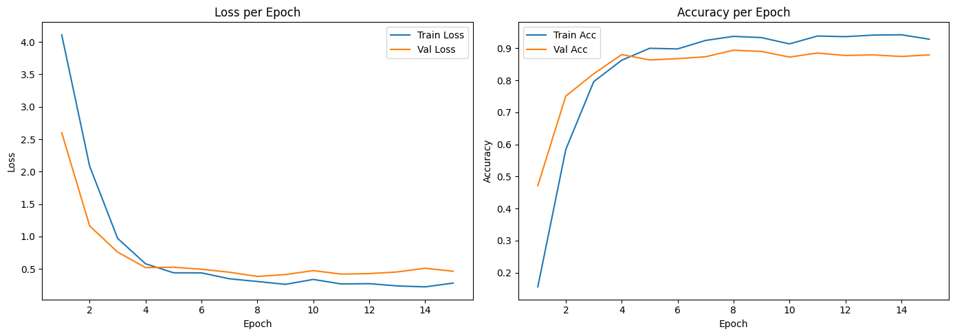
Validation accuracy (orange) peaks at epoch 8, then validation loss starts climbing again even as training loss keeps dropping, a textbook overfitting signature.

The weighted averages above hide a fair amount of variation between classes. Looking at the full 102-class classification report, several classes hit perfect precision and recall, 1.00, including bird of paradise and black-eyed susan. Others are much harder: mallow sits at 0.41 precision, japanese anemone at 0.46 recall. Visual similarity between certain flower classes is a likely factor here, along with the fairly small per-class training sample (around 10 images per class on average, given this dataset's official split).

📌 With 102 classes and uneven performance across them, accuracy alone can be misleading. A model can look good overall while struggling badly on specific classes. Per-class precision and recall catch what the average hides.

From Model to API with FastAPI

The model is trained and the best checkpoint (best.pt) is saved. Next: making it usable in the real world.

pip install fastapi uvicorn pillow torch torchvision

from fastapi import FastAPI, File, UploadFile
from fastapi.responses import JSONResponse
from PIL import Image
import torch
import torch.nn as nn
from torchvision import models, transforms
import io, json, urllib.request

app = FastAPI()
device = torch.device("cuda" if torch.cuda.is_available() else "cpu")

model = models.efficientnet_b1(weights=None)
num_ftrs = model.classifier[1].in_features
model.classifier = nn.Sequential(
    nn.Dropout(p=0.4, inplace=True),
    nn.Linear(num_ftrs, 102)
)
model.load_state_dict(torch.load('checkpoints/best.pt', map_location=device))
model = model.to(device)
model.eval()

transform = transforms.Compose([
    transforms.Resize(256),
    transforms.CenterCrop(224),
    transforms.ToTensor(),
    transforms.Normalize([0.485, 0.456, 0.406], [0.229, 0.224, 0.225])
])

with urllib.request.urlopen(
    "https://raw.githubusercontent.com/udacity/aipnd-project/master/cat_to_name.json"
) as resp:
    cat_to_name = json.load(resp)
class_names = [cat_to_name[str(i)] for i in range(1, 103)]

@app.post("/predict/")
async def predict(file: UploadFile = File(...)):
    try:
        image = Image.open(io.BytesIO(await file.read())).convert("RGB")
        input_tensor = transform(image).unsqueeze(0).to(device)

        with torch.no_grad():
            outputs = model(input_tensor)
            _, predicted = torch.max(outputs, 1)

        return JSONResponse(content={"predicted_class": class_names[predicted.item()]})
    except Exception as e:
        return JSONResponse(content={"error": str(e)}, status_code=400)

Three things that matter for serving this correctly:

1. The model architecture has to match training exactly, including the number of classes and the classifier structure. A mismatch can make load_state_dict fail outright, or worse, load successfully while producing wrong predictions with no error at all.

2. The transform has to match validation, not training. Use the same consistent Resize and CenterCrop, not random augmentation.

3. model.eval() and torch.no_grad() keep the model in pure inference mode.

Running the server:

uvicorn main:app --reload

curl -X POST "http://localhost:8000/predict/" -F "file=@path_to_your_image.jpg"

{"predicted_class": "sunflower"}

The model is now callable from any application, just send an image to the /predict/ endpoint.

Cheat Sheet

• [ ] Use a custom Dataset when labels don't come in a tidy folder structure

• [ ] Sort file listings manually when labels come from a separate array (like a .mat file)

• [ ] Augmentation applies to training data only, validation stays consistent

• [ ] A dataset's official split beats a custom random split for reproducibility

• [ ] Save two checkpoints: best.pt and last.pt

• [ ] Validation accuracy peaking then declining signals overfitting, not a bug

• [ ] Per-class precision and recall complement accuracy, especially with uneven class performance

• [ ] Serving architecture must match training architecture exactly

• [ ] Serving transform follows validation transform, not training

Test Your Understanding

1. Validation accuracy rises until epoch 8, then plateaus and drifts down through epoch 15. What does that mean?

Jawaban: Mild overfitting. The model keeps improving on training data, but its performance on unseen data stops improving past a certain point. This is why the best checkpoint, not the last one, gets used for deployment.

2. A model has 88% overall accuracy but only 46% recall on one class. What does that tell you?

Jawaban: The model is solid overall but specifically weak on that class, missing a large share of its actual samples. High overall accuracy can mask this when that class makes up a small fraction of the total data.

3. Why does the serving transform need to match validation, not training?

Jawaban: Training transforms include random augmentation meant to help the model generalize, not to represent an image "as-is." At inference time, images need consistent processing, matching exactly how the model was evaluated during validation.

4. Why does file order need manual sorting when labels come from a separate file?

Jawaban: Functions like os.listdir() don't guarantee consistent file ordering across systems. If labels assume files follow a specific numeric order, any mismatch can silently swap images and labels with no error raised.

5. What's the point of a dataset having an official train/val/test split from its original paper?

Jawaban: It makes results comparable to other research or experiments using the same dataset. A custom random split makes training numbers hard to compare across different runs or studies.

---

The two big questions left open at the end of the previous post, how to actually train the model and how to serve it, are answered here in full, from raw data to a callable API endpoint. Full code and the executed notebook are in the GitHub repo.

Part of an ongoing Computer Vision series.