Deep Learning & PyTorch: Neural Network Theory + Hands-On MNIST Classification

My mental model of deep learning used to be simple: feed it data, get a prediction, done. Turns out there's a much more grounded process behind that — artificial neurons that start knowing nothing, get things wrong repeatedly through backpropagation, and gradually learn to recognize patterns. These are my notes on how that actually works, from the fundamentals of neural networks to hands-on training a PyTorch model to recognize handwritten digits (MNIST).

Table of Contents

• What Is Deep Learning?

• Machine Learning vs Deep Learning

• Artificial Neurons — The Basics

• Neural Network Architecture

• Why PyTorch?

• Hands-On: Digit Classification with PyTorch

• Recap Checklist

• Mini Quiz

• Further Exercises

• Closing Thoughts

---

What Is Deep Learning?

Deep Learning is a subfield of Machine Learning that uses Artificial Neural Networks (ANNs) with many layers (multi-layer).

Two things set it apart from conventional ML:

• It can learn complex patterns from large, unstructured data.

• Feature representation happens automatically — features don't need to be manually engineered or selected like in conventional Machine Learning.

Deep Learning shows up heavily in Computer Vision, Natural Language Processing (NLP), Speech Recognition, and Recommendation Systems.

Machine Learning vs Deep Learning

The most fundamental difference is in the process flow:

	Flow
Machine Learning	Input → Feature Extraction (manual) → Classification (model) → Output
Deep Learning	Input → Feature Extraction + Classification (automatic, within the network) → Output

In ML, a human decides which features matter before feeding data into the model. In DL, feature extraction and classification happen together inside the network — which is why DL needs more data, but can also handle far more complex patterns.

Factor	Deep Learning	Machine Learning
Data Requirement	Needs large amounts of data	Can train on less data
Accuracy	Generally higher	Generally lower
Training Time	Longer	Shorter
Hardware Dependency	Needs a GPU for efficient training	Can train fine on CPU
Hyperparameter Tuning	Many tunable variations	Limited tuning options

Artificial Neurons — The Basics

Artificial neurons are inspired by biological ones: dendrites receive signals, the nucleus processes them, the axon sends signals onward. The math version:

• Each input (x₁, x₂, …, xₙ) is multiplied by its own weight (w).

• All the products are summed (Σ), then a bias (b) is added.

• The result passes through an activation function φ(.) to produce the output (y).

Z = W · X + b  →  Activation Function φ(Z)

🤔 Guess First: is ReLU typically used in the hidden layer or the output layer?

Answer: the hidden layer. ReLU (max(0, x)) is the standard activation between hidden layers because it's computationally cheap and helps the network learn non-linear patterns. For classification outputs, what's typically used is Softmax (multi-class, one label per sample) or Sigmoid per class (multi-label, multiple labels active at once) — not ReLU.

Neural Network Architecture

A Deep Neural Network is built from three types of layers:

1. Input Layer — receives the raw data as the initial input.

2. Hidden Layers — one or more hidden layers where complex patterns get learned; the more/deeper the layers, the more "deep" the network is.

3. Output Layer — produces the final result (prediction/classification).

Typically, every neuron in one layer connects to every neuron in the next (fully connected).

Why PyTorch?

A few reasons PyTorch is a solid choice for learning deep learning:

• Pythonic — the syntax feels natural and is easy for beginners to pick up.

• Widely used in both industry and academic research.

• Dynamic by design (define-by-run), which makes debugging much easier than with a static graph.

• Backed by a large open-source community, with a strong ecosystem: Torchvision, Torchtext, PyTorch Lightning, Torchserve.

The standard workflow for a Deep Learning project with PyTorch usually looks like this:

Load Dataset → Preprocessing → Build Model → Loss Function & Optimizer → Training Loop → Evaluation → Inference/Deployment

Let's put this workflow into practice.

---

Hands-On: Digit Classification with PyTorch

We'll build a simple neural network (SimpleNN) to recognize handwritten digits 0–9 from the MNIST dataset — the full pipeline, from loading data to a model ready for prediction.

1. Setup & Imports

import torch
import torch.nn as nn
import torch.optim as optim
from torch.utils.data import DataLoader
from torchvision import datasets, transforms, models

print('PyTorch version:', torch.__version__)

device = torch.device('cuda' if torch.cuda.is_available() else 'cpu')
print('Using device:', device)

# Set seed for reproducibility
SEED = 42
torch.manual_seed(SEED)
if torch.cuda.is_available():
    torch.cuda.manual_seed_all(SEED)

💡 torch.manual_seed() matters for reproducibility — without it, weight initialization and data shuffling are random, so results will vary slightly every time the notebook re-runs.

2. Load Dataset & DataLoader

transform = transforms.ToTensor()

train_dataset = datasets.MNIST(root='data', train=True, transform=transform, download=True)
test_dataset  = datasets.MNIST(root='data', train=False, transform=transform, download=True)

train_loader = DataLoader(train_dataset, batch_size=64, shuffle=True)
test_loader  = DataLoader(test_dataset, batch_size=64, shuffle=False)

len(train_dataset), len(test_dataset)

(60000, 10000)

The data is split into train (60,000 images) and test (10,000 images) right away — so evaluation later genuinely measures how well the model generalizes to data it's never seen, instead of data it's already memorized during training.

3. Looking at Sample Data

import matplotlib.pyplot as plt

images, labels = next(iter(train_loader))
print('Batch shape:', images.shape)
print('Labels:', labels[:10])

plt.figure()
plt.imshow(images[0].squeeze(), cmap='gray')
plt.title(f'Label: {labels[0].item()}')
plt.axis('off')
plt.show()

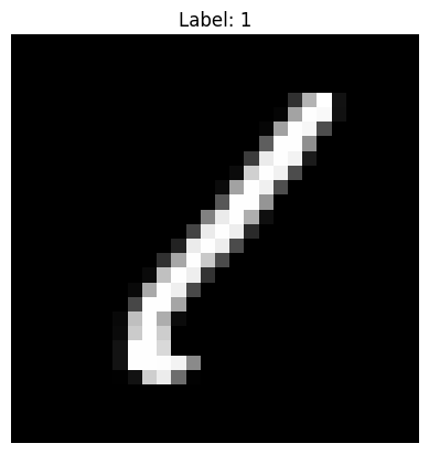
Each image is 28×28 pixels, grayscale (1 channel), labeled with a digit from 0 to 9.

4. Building a Simple Neural Network

class SimpleNN(nn.Module):
    def __init__(self):
        super().__init__()
        self.fc = nn.Sequential(
            nn.Flatten(), # out: 784 (28 * 28)
            nn.Linear(28 * 28, 128),
            nn.ReLU(),
            nn.Linear(128, 10)
        )

    def forward(self, x):
        return self.fc(x)

model = SimpleNN().to(device)
model

SimpleNN(
  (fc): Sequential(
    (0): Flatten(start_dim=1, end_dim=-1)
    (1): Linear(in_features=784, out_features=128, bias=True)
    (2): ReLU()
    (3): Linear(in_features=128, out_features=10, bias=True)
  )
)

The flow: Flatten turns the 28×28 image into a 784-length vector → the first Linear layer compresses it into 128 hidden features → ReLU adds non-linearity → the second Linear layer produces 10 outputs (one per digit, 0–9).

Notice the model does not end with a Softmax layer. That's intentional — nn.CrossEntropyLoss(), used in the next step, already applies log-softmax internally. Adding a manual Softmax here would apply that activation twice, which would mess up training.

5. Loss Function & Optimizer

criterion = nn.CrossEntropyLoss()
optimizer = optim.Adam(model.parameters(), lr=1e-3)

6. Training Loop

def train(model, loader, criterion, optimizer, device):
    model.train()
    running_loss = 0.0
    for images, labels in loader:
        images, labels = images.to(device), labels.to(device)

        outputs = model(images)
        loss = criterion(outputs, labels)

        optimizer.zero_grad()
        loss.backward()
        optimizer.step()

        running_loss += loss.item() * images.size(0)

    return running_loss / len(loader.dataset)

num_epochs = 10
for epoch in range(num_epochs):
    loss = train(model, train_loader, criterion, optimizer, device)
    print(f'Epoch [{epoch+1}/{num_epochs}] - Loss: {loss:.4f}')

Epoch [1/10] - Loss: 0.3421
Epoch [2/10] - Loss: 0.1532
Epoch [3/10] - Loss: 0.1044
Epoch [4/10] - Loss: 0.0789
Epoch [5/10] - Loss: 0.0630
Epoch [6/10] - Loss: 0.0508
Epoch [7/10] - Loss: 0.0417
Epoch [8/10] - Loss: 0.0337
Epoch [9/10] - Loss: 0.0284
Epoch [10/10] - Loss: 0.0238

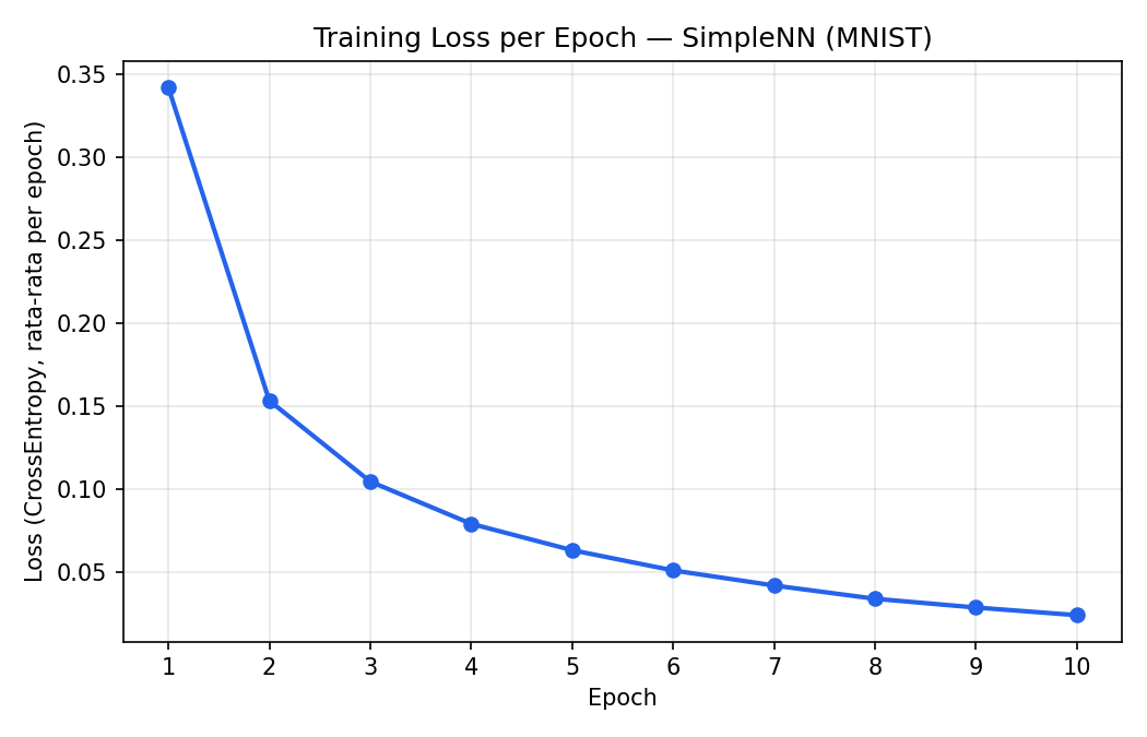
Loss drops steadily from 0.3421 in the first epoch to 0.0238 in the last — a good sign the model is genuinely learning, not stagnating or getting worse.

A technical note: running_loss += loss.item() * images.size(0), divided by len(loader.dataset) at the end, gives the average loss over a full epoch — not just the loss from the last batch. Printing loss.item() at the end of the loop alone would only reflect the very last batch, which can be misleading as a progress indicator.

7. Evaluating Accuracy on Test Data

def evaluate(model, loader, device):
    model.eval()
    correct, total = 0, 0
    with torch.no_grad():
        for images, labels in loader:
            images, labels = images.to(device), labels.to(device)
            outputs = model(images)
            _, preds = outputs.max(1)
            total += labels.size(0)
            correct += (preds == labels).sum().item()
    return correct / total

test_acc = evaluate(model, test_loader, device)
print(f'Test accuracy: {test_acc:.4f}')

🤔 Guess First: how accurate do you think this simple model (just 1 hidden layer, 10 epochs) is on test data?

Answer: 97.86%. Pretty impressive for such a simple architecture — it shows MNIST is a relatively "easy" benchmark dataset, and shows a basic fully-connected network is already strong enough for image classification tasks that aren't too complex (at least for this one experiment — not necessarily true across every dataset).

model.eval() and torch.no_grad() matter here: eval() switches the model's mode (relevant if there were layers like Dropout/BatchNorm), and no_grad() disables gradient computation since evaluation doesn't need backward() — making the process faster and more memory-efficient. One thing to watch closely: loader here must be test_loader, not train_loader — evaluating on the same data used for training would produce a biased accuracy that doesn't reflect the model's actual ability to generalize.

8. Inference on a Single Image

model.eval()
image, label = test_dataset[0]
plt.figure()
plt.imshow(image.squeeze(), cmap='gray')
plt.title(f'Ground truth: {label}')
plt.axis('off')
plt.show()

with torch.no_grad():
    x = image.unsqueeze(0).to(device)
    output = model(x)
    pred = output.argmax(1).item()

print('Model prediction:', pred)

	Value
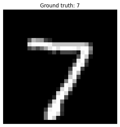
Ground truth	7
Model prediction	7
Status	✅ Correct

image.unsqueeze(0) adds a batch dimension up front (turning [1, 28, 28] into [1, 1, 28, 28]) — because the model expects data in batch form, even when we only want a prediction for a single image.

9. Saving & Reloading the Model

There are two ways to save a model in PyTorch:

# Option 1: save only the model weights (most common, recommended)
torch.save(model.state_dict(), "model_mnist.pth")

# Option 2: save the entire model object (rarely used, but still possible)
torch.save(model, "full_model_mnist.pth")

To reload the model from saved weights:

model = SimpleNN().to(device)
model.load_state_dict(torch.load("model_mnist.pth", map_location=device))
model.eval()

💡 map_location=device matters if you save a model from a GPU machine and want to load it on a machine without a GPU (or vice versa) — without it, torch.load() can throw an error trying to map tensors to a device that isn't available.

---

Recap Checklist

• [ ] Understand the difference between ML (manual feature extraction) and DL (automatic)

• [ ] Can explain the basic neuron formula: Z = W·X + b → φ(Z)

• [ ] Know the three layer types: input, hidden, output

• [ ] Understand why ReLU belongs in hidden layers, not the output

• [ ] Can lay out the PyTorch workflow: dataset → model → loss/optimizer → training loop → evaluation → inference

• [ ] Understand why model.eval() + torch.no_grad() are used during evaluation/inference

• [ ] Know why evaluation should use test_loader, not train_loader

• [ ] Can save and reload a model with state_dict()

Mini Quiz

1. Why doesn't the SimpleNN model above end with a Softmax layer?

Because nn.CrossEntropyLoss() in PyTorch already applies log-softmax internally. Adding a manual Softmax to the model would apply that activation twice, which disrupts training.

2. What happens if you evaluate the model using train_loader instead of test_loader?

The resulting accuracy would be biased — reflecting how well the model "memorized" the training data, rather than how well it generalizes to new, unseen data.

3. What does torch.no_grad() do during evaluation?

It disables gradient computation, since evaluation/inference never calls backward(). This makes the process faster and more memory-efficient than keeping gradient tracking on.

Further Exercises

To explore further from this notebook:

1. Change the hidden layer size from 128 to 256 or 64 — observe the effect on accuracy.

2. Add a new fully-connected layer (3 layers instead of 2).

3. Swap the optimizer from Adam to SGD, and compare convergence speed.

4. Add Dropout to the model and observe its effect on overfitting.

Closing Thoughts

The thing that stuck with me most from this material: deep learning isn't magic — it's just a simple neuron (Z = W·X + b) stacked in layers, trained through a highly structured trial-and-error process (forward pass → compute loss → backward pass → update weights). What makes it powerful is the scale and repetition, not the complexity of any single neuron.

The full, end-to-end verified notebook is available on this GitHub repo.

---

Part of my AI Engineering learning notes series — AI Notes & Engineering