
Hands-On Data Preprocessing with Python: From Missing Values to PCA

Learning notes with code that actually runs — six core data preprocessing techniques you'll reach for before feeding data into a Machine Learning model, backed by real execution output instead of made-up numbers.
There's a saying that gets repeated a lot in data science: "80% of AI work is data, not the model" (the exact number varies by source, but the general point tends to hold up). What people usually mean is this part of the pipeline: checking for missing values, catching and handling outliers, turning categories and text into numbers, compressing dimensions, and keeping a version history of your data. Every technique below was run with actual Python code (Pandas + Scikit-learn), against two kinds of data — a real 10,000-row customer dataset, and a few small synthetic examples to make the concepts concrete.
Note on the code blocks: variable names are kept exactly as they were in the original notebook (Indonesian words like
nama,umur,gaji,batas_bawah) rather than translated, so the code here is byte-for-byte reproducible against the source. Only the surrounding explanation is in English.
📂 The full notebook (already executed end-to-end, dataset included) is on GitHub: github.com/arielshakaramiro/data-preprocessing-praktik-arielshakaramiro
Table of Contents
1. Data Collection & Storage: Quick Concept
Before diving into practice, there are two types of data worth knowing:
Unstructured Data — data with "free-form" shape, like images, text, or audio. Humans can grasp its meaning directly without any special structure (e.g., we instantly recognize a picture of a cat).
Structured Data — data neatly organized into rows and columns, like transaction records or customer data. Its meaning depends heavily on business context, so it's not always understandable "at a glance" to a non-expert.
Both types need storage that's secure, easily accessible, and versionable (keeps a history of changes) — this versioning concept is covered further in section 7.
2. Missing Values: Check First, Don't Assume
There are two common ways to handle missing (NaN) values:
Dropna — remove rows/columns with missing data. Works well when only a small amount is missing.
Fillna — fill the gap with a substitute: mean, median, or mode (the most frequent value).
The step beginners skip most often: check first, don't assume the data is dirty.
sample_data = pd.read_csv('customers-10000.csv')
print(sample_data.isnull().sum())
(The original code loads the dataset from a Google Drive link; it's written here as a local file for easy reproduction — the content is identical, a public 10,000-row dataset from Datablist.)
Real execution result on the customer dataset (10,000 rows, 12 columns — Index, Customer Id, First Name, Last Name, Company, City, Country, Phone 1, Phone 2, Email, Subscription Date, Website):
Missing values per column: 0 (every column, 0.0%)
🤔 Guess First: How much of a public-facing customer dataset like this do you think is typically missing?
Reveal Answer
In this case: 0% — this is a synthetic dataset generated with Faker for practice purposes, so it was built clean on purpose, with no missing values at all. That's actually the real lesson here: never assume a dataset is "obviously dirty." Always run
.isnull().sum()first before deciding on a strategy — if it turns out clean, you just saved yourself time; if something is missing, you know exactly which column needs attention.
To actually see both handling techniques in action, a tiny synthetic dataset was built with intentional gaps:
data = {
    'nama': ['Andi', 'Budi', 'Citra', 'Dewi', 'Eka'],
    'umur': [25, np.nan, 30, 22, np.nan],
    'gaji': [5000000, 6000000, np.nan, 4500000, 5200000]
}
df = pd.DataFrame(data)
| nama | umur | gaji |
|---|---|---|
| Andi | 25 | 5,000,000 |
| Budi | NaN | 6,000,000 |
| Citra | 30 | NaN |
| Dewi | 22 | 4,500,000 |
| Eka | NaN | 5,200,000 |
(nama = name, umur = age, gaji = salary — kept in the original language since that's the actual column names in the code.)
Missing count and percentage per column (real output of df.isnull().sum() and df.isnull().sum() / len(df) * 100):
| Column | Missing Count | Percentage |
|---|---|---|
| nama | 0 | 0% |
| umur | 2 | 40% |
| gaji | 1 | 20% |
Option 1 — dropna():
df_dropped = df.dropna()
Budi, Citra, and Eka all get dropped since each has one empty cell — 5 rows shrink down to 2. Effective when the missing amount is small and those rows aren't critical; wasteful when the data is valuable but just happens to have one blank column.
Option 2 — fillna() with mean/median:
df_filled = df.copy()
df_filled['umur'] = df_filled['umur'].fillna(df_filled['umur'].mean())
df_filled['gaji'] = df_filled['gaji'].fillna(df_filled['gaji'].median())
Missing ages get filled with the average of the ones present, and missing salaries get filled with the median. (Added context beyond the original code: median is generally chosen for salary because it's more robust against extreme values than the mean — this will make more sense after the outlier section below.)
3. Detecting & Handling Outliers with IQR
An outlier is a data point that sits far outside the majority. The decision rule:
Outliers that are rare and don't impact the business → safe to drop.
Outliers that do disrupt business processes → don't just drop them, handle them more carefully (at production scale, one advanced approach is an Autoencoder — a small model that learns the pattern of normal data, so data that deviates far from that pattern produces a large reconstruction error and can be flagged as an outlier).
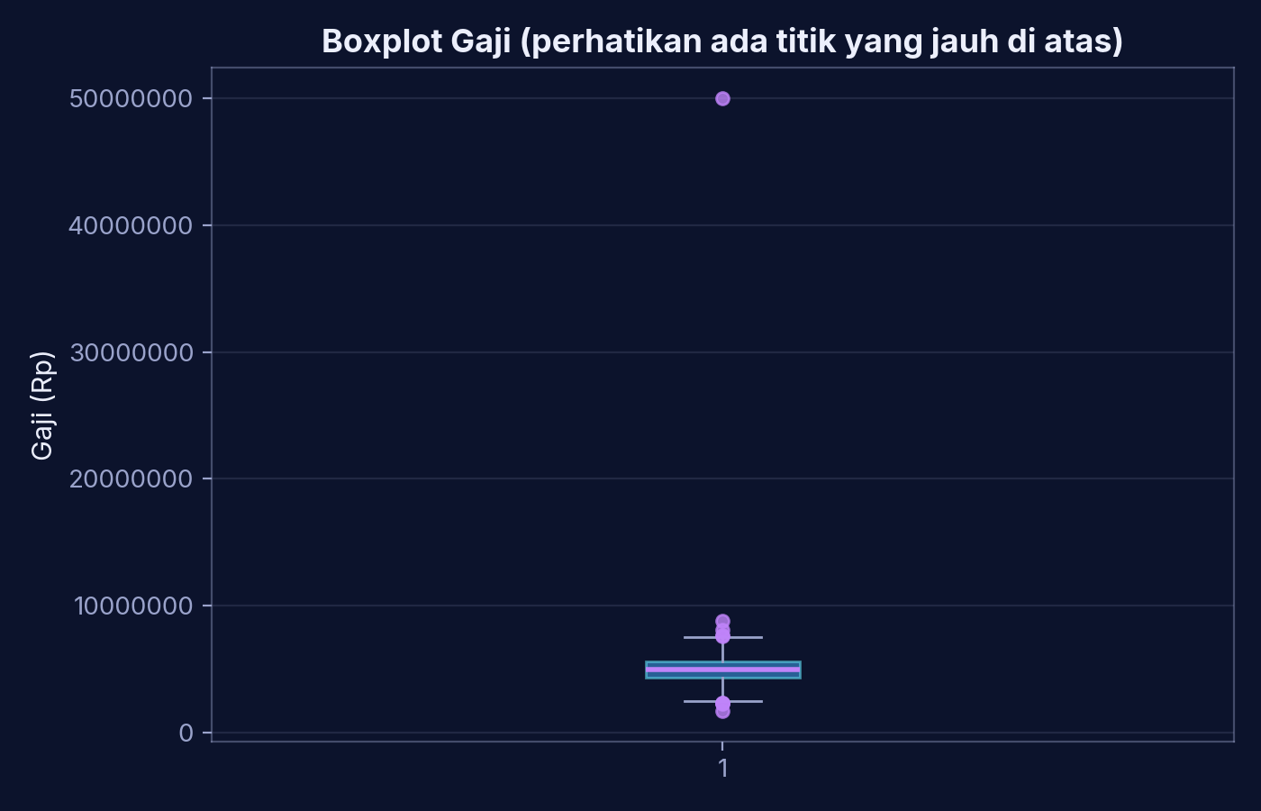
For beginners, one of the most common and straightforward methods is IQR (Interquartile Range). The simulation: 1,000 normally-distributed salary (gaji) values (mean Rp5,000,000, standard deviation Rp1,000,000), with 1 extreme outlier of Rp50,000,000 injected on top.
np.random.seed(42)
gaji = np.random.normal(5000000, 1000000, 1000).tolist()
gaji.append(50000000)  # outlier: a salary far larger than the rest
df_gaji = pd.DataFrame({'gaji': gaji})
A quick look before computing anything — the boxplot code:
plt.figure(figsize=(6, 4))
plt.boxplot(df_gaji['gaji'])
plt.title('Boxplot Gaji (perhatikan ada titik yang jauh di atas)')
plt.ylabel('Gaji')
plt.show()
(The title/label strings are left in Indonesian, exactly as they were actually run — "Boxplot Gaji (perhatikan ada titik yang jauh di atas)" means "Salary boxplot, notice the point far above.")
Then the bounds get computed mathematically with IQR:
Q1 = df_gaji['gaji'].quantile(0.25)
Q3 = df_gaji['gaji'].quantile(0.75)
IQR = Q3 - Q1
batas_bawah = Q1 - 1.5 * IQR
batas_atas = Q3 + 1.5 * IQR

outliers = df_gaji[(df_gaji['gaji'] < batas_bawah) | (df_gaji['gaji'] > batas_atas)]
(batas_bawah = lower bound, batas_atas = upper bound.)
Real execution results (with random seed 42, so the numbers are reproducible on a re-run):
| Metric | Value |
|---|---|
| Q1 (lower quartile) | Rp4,353,427 |
| Q3 (upper quartile) | Rp5,648,710 |
| IQR | Rp1,295,283 |
| Lower bound | Rp2,410,503 |
| Upper bound | Rp7,591,634 |
| Outliers detected | 9 out of 1,001 rows |
🤔 Guess First: Only 1 fake outlier (Rp50M) was injected. Do you think IQR flags exactly 1 outlier too, or could it be more?
Reveal Answer
It flagged 9 outliers, not just 1. Besides the injected Rp50M value, 8 other data points — pure products of the normal distribution, not intentional — happened to land outside the 1.5×IQR range, and they sit on both sides: 4 below the lower bound (roughly Rp1.76M–2.38M) and 4 above the upper bound (roughly Rp7.63M–8.85M). The lesson: the IQR method is purely statistical, it has no idea which values are "intentional anomalies" and which are just "extreme by coincidence" due to the natural spread of the data. That's why, before dropping anything IQR flags, it's still worth checking the business context — an Rp8M salary in this dataset could genuinely be a director's valid salary, not a data-entry mistake, and an Rp1.8M salary might just be an intern.
After removal:
df_bersih = df_gaji[(df_gaji['gaji'] >= batas_bawah) & (df_gaji['gaji'] <= batas_atas)]
The clean remainder: 992 out of 1,001 rows.
4. Feature Engineering: Turning Categories into Numbers
Machine Learning models only understand numbers, not text categories like "Apple" or "Chicken." Two common ways to convert them:
| Technique | How It Works | When to Use |
|---|---|---|
| Label Encoding | Each category gets one unique number | Categories with a natural order/rank (low–medium–high) |
| One Hot Encoding | Each category becomes its own 0/1 column | Categories with no order (food names, cities, etc.) — the safer default |
Example data:
food = pd.DataFrame({
    'Food Name': ['Apple', 'Chicken', 'Broccoli'],
    'Calories': [95, 231, 50]
})
| Food Name | Calories |
|---|---|
| Apple | 95 |
| Chicken | 231 |
| Broccoli | 50 |
Label Encoding (real LabelEncoder output):
| Food Name | Calories | Categorical # |
|---|---|---|
| Apple | 95 | 0 |
| Chicken | 231 | 2 |
| Broccoli | 50 | 1 |
Notice the numbers follow alphabetical order (Apple=0, Broccoli=1, Chicken=2) — not calories or any meaningful ranking. This is a classic source of bugs: applied to categories with no real order, a model can "read" Chicken (2) as somehow twice as large or important as Broccoli (1), when it's really just an alphabetical index.
One Hot Encoding (real pd.get_dummies output):
| Calories | Food Name_Apple | Food Name_Broccoli | Food Name_Chicken |
|---|---|---|---|
| 95 | 1 | 0 | 0 |
| 231 | 0 | 0 | 1 |
| 50 | 0 | 1 | 0 |
No implied ordering — each category gets its own column. The trade-off: with hundreds or thousands of categories (postal codes, for example), the column count can explode.
5. Text Preprocessing: Bag of Words & TF-IDF
Just like categories, text also needs to become a numeric vector (vectorization). Example corpus (3 short Indonesian sentences):
corpus = [
    "rumah ini bagus",        # d1 - "the house is nice"
    "rumah saya makan nasi",  # d2 - "my house, I eat rice"
    "saya makan nasi"         # d3 - "I eat rice"
]
Bag of Words — counts how many times each word appears in each document:
vectorizer = CountVectorizer()
bow_matrix = vectorizer.fit_transform(corpus)

bow_df = pd.DataFrame(
    bow_matrix.toarray(),
    columns=vectorizer.get_feature_names_out(),
    index=['d1', 'd2', 'd3']
)
Real execution result (bow_df):
| bagus | ini | makan | nasi | rumah | saya | |
|---|---|---|---|---|---|---|
| d1 | 1 | 1 | 0 | 0 | 1 | 0 |
| d2 | 0 | 0 | 1 | 1 | 1 | 1 |
| d3 | 0 | 0 | 1 | 1 | 0 | 1 |
BoW has a weakness: words that appear in every document get counted as heavily as any other word, even though they don't help tell documents apart.
TF-IDF (Term Frequency–Inverse Document Frequency) fixes this — words that show up across many documents get a lower weight, while rarer, more unique words get a higher weight:
tfidf_vectorizer = TfidfVectorizer()
tfidf_matrix = tfidf_vectorizer.fit_transform(corpus)

tfidf_df = pd.DataFrame(
    tfidf_matrix.toarray(),
    columns=tfidf_vectorizer.get_feature_names_out(),
    index=['d1', 'd2', 'd3']
).round(3)
Real execution result (tfidf_df, rounded to 3 decimals):
| bagus | ini | makan | nasi | rumah | saya | |
|---|---|---|---|---|---|---|
| d1 | 0.623 | 0.623 | 0.000 | 0.000 | 0.474 | 0.000 |
| d2 | 0.000 | 0.000 | 0.500 | 0.500 | 0.500 | 0.500 |
| d3 | 0.000 | 0.000 | 0.577 | 0.577 | 0.000 | 0.577 |
🤔 Guess First: "rumah" appears in both d1 and d2, while "bagus" only appears in d1. Do you think the TF-IDF weight of "bagus" in d1 is higher or lower than "rumah" in d1?
Reveal Answer
Higher (0.623 vs 0.474). "rumah" appears in 2 out of 3 documents, so it's considered less distinctive → its weight gets pulled down. "bagus" only appears in 1 document (d1) → it's considered more distinctive for that document → its weight is higher. That's the core idea behind IDF: the rarer a word is across the whole corpus, the more "distinguishing power" it carries for the document it appears in.
💡 Beyond the core material: There's a more advanced method called Word2Vec — a small neural network that learns word meaning from surrounding words, rather than just counting frequency. The result: words with similar meanings end up with vector positions close to each other (for instance, "King" and "Queen" end up close together along a dimension roughly representing "power/rank"). This is a natural next step after mastering BoW and TF-IDF.
6. Reducing Dimensions with PCA
Sometimes data has too many columns/features, making it hard to visualize or slowing a model down. PCA (Principal Component Analysis) compresses data into fewer dimensions while preserving as much of the important information as possible.
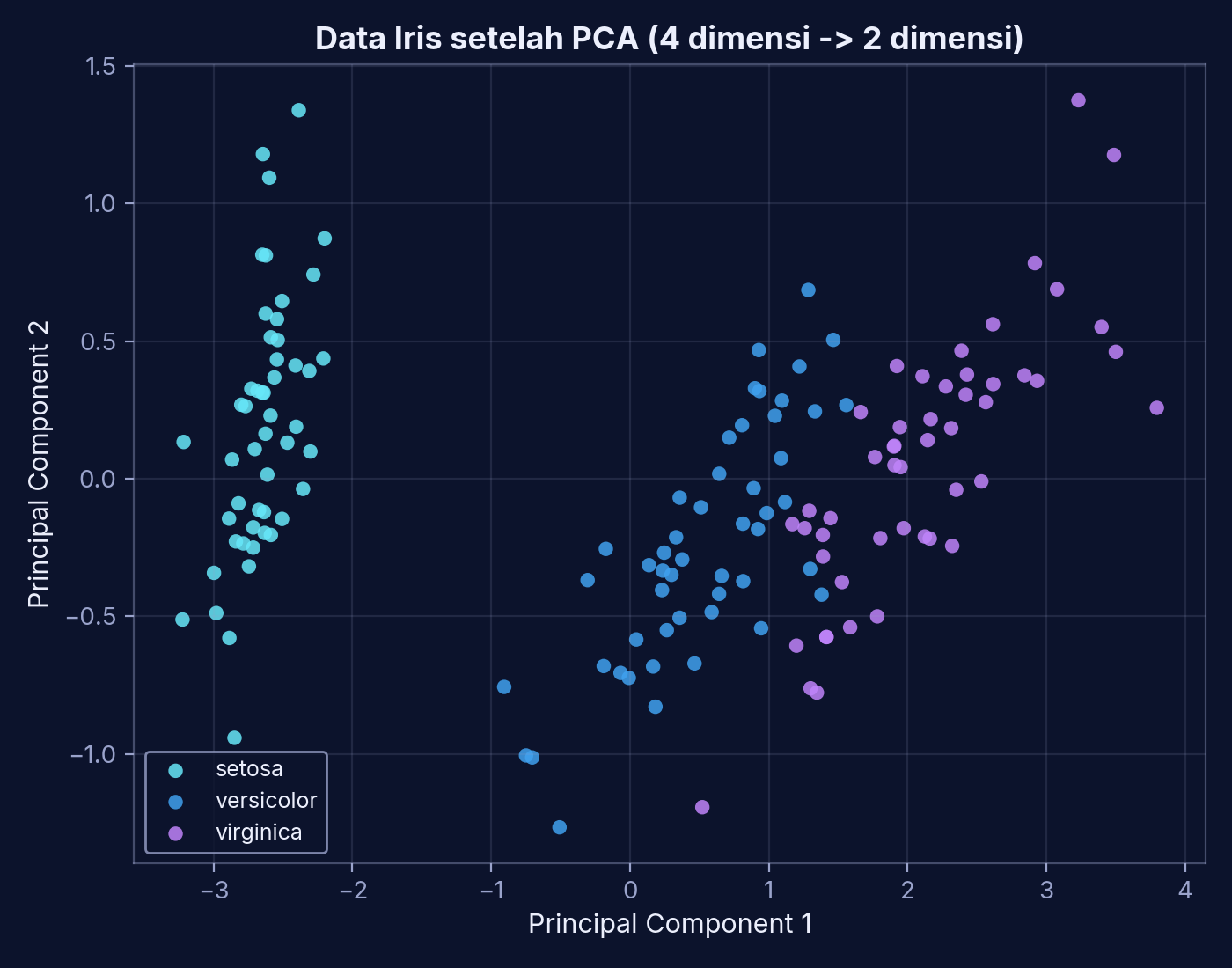
Example: the Iris flower dataset (4 features — petal/sepal length & width) compressed down to 2 dimensions.
iris = load_iris()
X = iris.data   # 4 features: petal/sepal length & width
y = iris.target # flower species

pca = PCA(n_components=2)
X_pca = pca.fit_transform(X)

plt.figure(figsize=(6, 5))
scatter = plt.scatter(X_pca[:, 0], X_pca[:, 1], c=y, cmap='viridis')
plt.xlabel('Principal Component 1')
plt.ylabel('Principal Component 2')
plt.title('Data Iris setelah PCA (4 dimensi -> 2 dimensi)')
plt.legend(handles=scatter.legend_elements()[0], labels=list(iris.target_names))
plt.show()

print(f"Dimensi awal: {X.shape[1]} fitur")
print(f"Dimensi setelah PCA: {X_pca.shape[1]} fitur")
print(f"Informasi yang berhasil dijaga: {pca.explained_variance_ratio_.sum()*100:.1f}%")
(The plot title and print labels are left exactly as run — "Dimensi awal" = original dimensions, "Dimensi setelah PCA" = dimensions after PCA, "Informasi yang berhasil dijaga" = information preserved.)
Output of the three print lines above, plus the per-component breakdown (pca.explained_variance_ratio_):
| Metric | Value |
|---|---|
| Original dimensions | 4 features |
| Dimensions after PCA | 2 features |
| Variance kept by PC1 | 92.5% |
| Variance kept by PC2 | 5.3% |
| Total information preserved | 97.8% |
In other words: the original 4 columns get cut down to 2, but only about 2.2% of the information is lost — a trade-off that's usually well worth it for visualization or speeding up model training. The scatter plot also shows it clearly: the setosa species (cyan) is already cleanly separated from the other two even with just 2 dimensions, while versicolor (blue) and virginica (purple) overlap a bit in the middle.
7. The Data Versioning Concept
A simple analogy: saving a document as report_v1, then report_v2 after a revision — so if the new version turns out wrong, you can still go back to the old one. Data versioning applies the same idea to datasets.
Why it matters for Machine Learning:
If a model suddenly gets worse after a data update, you can roll back to the previous data version.
Model development becomes easier to track — which matters a lot for debugging and audits.
Commonly used real-world tools:
| Category | Example Tools |
|---|---|
| Dataset versioning | DVC, GitLab |
| Annotation + versioning | CVAT, Roboflow, SuperAnnotate |
| Experiment tracking | MLflow, Neptune.ai, Weights & Biases |
The simplest possible simulation: saving each dataset "version" as a separate file.
import os
os.makedirs('data_versions', exist_ok=True)

df_v1 = pd.DataFrame({'nama': ['Apple', 'Chicken'], 'kalori': [95, 231]})
df_v1.to_csv('data_versions/dataset_v1.csv', index=False)

df_v2 = df_v1.copy()
df_v2.loc[len(df_v2)] = ['Broccoli', 50]
df_v2.to_csv('data_versions/dataset_v2.csv', index=False)
(kalori = calories.)
dataset_v1.csv holds 2 rows (Apple, Chicken); dataset_v2.csv holds 3 rows (Apple, Chicken, Broccoli) — a small ("micro") change gets saved as a separate file, so the old version stays accessible at any time.
⚠️ Transparency note: the example above is just a concept simulation using manually separated files — it's not how real versioning tools like DVC actually work under the hood (they use content hashing and storage separate from Git). It's simplified here so the core idea is easy to grasp without extra installation.
8. Summary & Next Steps
| Stage | What Was Covered |
|---|---|
| Missing Values | dropna() and fillna() |
| Outliers | IQR detection + boxplot |
| Feature Engineering | Label Encoding & One Hot Encoding |
| Text Preprocessing | Bag of Words & TF-IDF |
| Dimensionality Reduction | PCA |
| Data Versioning | The concept of keeping a dataset's version history |
A few next steps worth trying on your own:
Swap in your own dataset instead of the examples above.
Explore the
gensimlibrary to go deeper into Word2Vec.Try an open-source tool like DVC for real, production-grade data versioning.
9. Cheat Sheet: Preprocessing Checklist
[ ] Check for missing values first with
.isnull().sum()before assuming the data is dirty[ ] Small, non-critical gaps →
dropna(); valuable data or large gaps →fillna()(mean/median/mode)[ ] Detect outliers with IQR, but check the business context before dropping — a statistical outlier isn't automatically a data error, and outliers can show up on either side of the distribution
[ ] Ordered categories (low–medium–high) → Label Encoding; unordered categories → One Hot Encoding
[ ] Short/simple text → Bag of Words; need to distinguish "distinctive" words from common ones → TF-IDF
[ ] Too many features → consider PCA, and check how much information is actually retained
[ ] Keep a version history of your data (not just your code) — so you can roll back if a model suddenly gets worse
10. Quiz Check
1. Why check .isnull().sum() first, before jumping straight to dropna/fillna?
Because not every dataset is automatically "dirty" — in the customer dataset example above, the result was 0% missing values across every column. Skipping the check and applying a cleaning strategy anyway risks wasting time (or worse, discarding perfectly fine data) on a problem that didn't actually exist.
2. Why was the missing salary filled with the median instead of the mean?
The median is more robust against extreme values/outliers than the mean. If one salary is far larger than the rest, the mean gets pulled upward and becomes less representative, while the median stays stable near the center of the data.
3. IQR flagged 9 outliers even though only 1 was injected intentionally, and they sat on both sides of the distribution. What does that mean?
Statistical methods like IQR have no way of distinguishing "intentionally anomalous" data from values that just happen to sit at either tail of a normal distribution. Everything outside the 1.5×IQR range gets flagged the same way. So outlier detection results still need to be verified against business context before deciding whether to drop or keep them.
4. When should you avoid Label Encoding for categories like city names or food names?
When the category has no natural order/ranking. Label Encoding assigns sequential numbers (0, 1, 2, ...) that a model can accidentally "read" as a mathematical relationship — for instance, treating category 2 as "greater than" category 1, when that ordering was really just alphabetical coincidence. One Hot Encoding is the safer choice here.
5. Why do words that appear in many documents get a lower TF-IDF weight?
Because TF-IDF's whole purpose is measuring how distinctive a word is for telling one document apart from another. A word that shows up in most or all documents (like "rumah" here) doesn't help distinguish between them much, so its IDF weight is pulled down. A rarer word carries more information about the specific document it appears in, so it gets a higher weight.
Every number and chart in this post comes from actually running the code (not a manual simulation), with the random seed for the outlier section noted so the results are reproducible.